The File Drawer
The minimum post-stratification weight in a simple-random-sample equals the response rate
As my first post on the File Drawer, I wanted to share a survey statistics result that surprised me and that I haven’t seen derived before. At the very least, I know that this result is not used in any applied weighting work that I’ve seen.
How differential nonresponse ruins the law of large numbers
Random samples have fantastic statistical properties. As the sample size increases, the law of large numbers guarantees that your estimate will converge on the true population value. However, that statement assumes that the gap between an estimate and population value is entirely due to sampling variability. In practice, all estimates suffer from bias as well as random error.
One form of bias comes from differential non-response. Suppose I claim that 30% of the population holds a deep hatred of surveys and that their highest political priority is to throw pollsters in prison. This claim is actually quite hard to disprove with survey data. If you come back to me with a survey with a typical response rate (around 50% for high quality probability surveys and as low as 6% for phone polls) that shows only 1% of the public wants to imprison pollsters, I’ll just point out that you haven’t accounted for differential non-response in creating this estimate. Maybe the the 30% of anti-survey zealots refuse to take surveys.
If the survey’s response rate is above 70%, though, then you can disprove my 30% claim. If the survey has a 90% response rate, there can’t be enough non-responding anti-survey extremists to make up the difference between 1% and 30%.
While this usage of the response rates is unlikely to come up much in the real world, the response rate of a survey has a surprising analytic relationship to the logical constraints of post-stratification survey weights. Post-stratification weights attempt to correct for non-response bias by counting responses from respondents from low response rate groups as if they represented more respondents and counting responses from high response rate groups as if they represented a smaller number of respondents. These post-stratification weights attempt to correct for known differences between the survey sample and known facts about the population such as the proportion of women, how many people live in each region and how many people are different ages.
In short, the most overrepresented a respondent can be is if the subgroup they represent (even if we don’t know what defines that subgroup) has a 100% response rate while the survey as a whole has some lower response rate \(RR_{total}\). Interestingly, it turns out that in this situation, the weight for a respondent in this maximally overrepresented subgroup is equal to the response rate for the survey as a whole. Since all possible subgroups (however, defined) must have a response rate of 100% or below, this situation represents the lower possible bound of a respondent’s probability weight for a simple random sample (e.g. no stratification or selection weights etc.). And the best part–accounting for this constraint in weighting algorithms should improve the bias and efficiency of weights!
Proving that the minimum survey weight for a respondent is equal to the response rate
Feel free to skip this section if you’re happy to believe me, but the maths is actually pretty straightforward.
Let’s define the subgroup that a respondent, \(i\), belongs to as \(group[i]\), the set of people who took the survey as \(S\), and the set of people in the population as \(P\). I define the proportion of the sample who are in the respondent’s, \(i\), subgroup as:
\[ s_i = \frac{| \{ j|group[j]=group[i] \wedge j \in S \} |}{|S|} \] and the proportion of the population who are part of the respondent’s subgroup as:
\[p_i = \frac{| \{ j|group[j]=group[i] \} |}{|P|}\] The proportion of the sample who are in the respondent’s subgroup can be expressed by multiplying the response rate for the subgroup \(RR_{group[i]}\) then dividing by the total response rate for the sample \(RR_{total}\):
\[ s_i = \frac{p_i \cdot RR_{group[i]}}{RR_{total}} \]
Since we are assuming the worst case scenario for a subgroup being overrepresented, we set \(RR_{group[i]}=1\), so that:
\[ s_i = \frac{p_i}{RR_{total}} \]
The true weight \(TrueWeight_i\) for a respondent is defined by dividing the target proportion of the population \(p_i\) in the respondent’s subgroup by the proportion of the sample in the subgroup:
\[ TrueWeight_i = \frac{p_i}{s_i} \]
Assuming that all subgroups in the population are present within the sample (i.e. there are no empty cells), these true weights would exactly balance the sample to the population.
We can substitute in our equation for the sample proportion above into the true weight formula
\[ TrueWeight_i = \frac{p_i}{\frac{p_i}{RR_{total}} }\\ \\ = RR_{total} \]
So in the case where a subgroup (which may be defined by any number of arbitrary observed or unobserved characteristics) is maximally overrepresented in a survey, a respondent in that subgroup should get a post-stratification weight equal to the survey response rate.
Pretty neat, right?
So what?
Does it make a difference if we use this constraint? Let’s use an example with fictional numbers.
So let’s suppose there are two important variables we’re interested in and that they’re also the only things that matter for response rates. In this case, we’ll say they are whether someone is vaccinated and whether they are rich or poor.
Let’s say we know from official figures that exactly 51% of the population are vaccinated and from different official sources that exactly 49% of the population are rich.
We run a simple random sample probability survey to look at how these two things are related and get a 50% response rate. However, our unweighted survey data says that 76% of people are vaccinated and that 81% are rich, so we know that there must be differential response by these two variables.1
Because this is fake data, we actually know what the response rates are in each group:
| Vaccinated | Unvaccinated | |
|---|---|---|
| Rich | 100 | 55 |
| Poor | 38 | 5 |
as well as the true proportions of the population who are in each combination of wealth and vaccination status:
| Vaccinated | Unvaccinated | |
|---|---|---|
| Rich | 30 | 19 |
| Poor | 21 | 31 |
So we have survey data with differential non-response and marginal targets for two key variables but no target information about their joint distribution. This is the classic situation where researchers use the raking algorithm to create weights. This algorithm iteratively adjusts the weight for each variable so that the weights reproduce the correct population proportions for that weight.
This works by using the current weights (which starts off as 1 for all respondents in the case of a simple random sample) to calculate the weighted proportion of respondents in a particular group A: \(WeightedSample_{A}\). The weights for respondents in group A are then multiplied by the proportion of the population in group A (\(Population_{A}\)) then divided by \(WeightedSample_{A}\).
So the new weight for a respondent, \(i\), who is a member of group A is:
\[ NewWeight_i = \frac{Population_{A}}{WeightedSample_{A}} \cdot OldWeight_i \] Similarly the new weight for a respondent, \(j\) who is not in group A is:
\[ NewWeight_j = \frac{Population_{\neg A}}{WeightedSample_{\neg A}} \cdot OldWeight_j \]
Once the new weights are created, the sample will now return the correct proportions in terms of being in group A or not.
At this stage, we repeat the same process with the next variable we want to weight to. However, because the weights are adjusted for each variable sequentially, the sample will be unbalanced by later reweighting steps. Fortunately though, the weights will converge to give the correct proportions for all variables simply by repeating this procedure multiple times.
We can see in the following plot that the raw sample does a very bad job at representing the size of each subgroup properly. The standard raking algorithm improves the situation substantially, but it underestimates the proportion of poor unvaccinated people and–perhaps more surprisingly–the proportion of rich vaccinated people.
However, when I add in the constraint that the minimum weight in a cell is equal to the overall response rate for the survey (0.5), the proportions in the weighted sample are corrected to exactly match the true proportions.
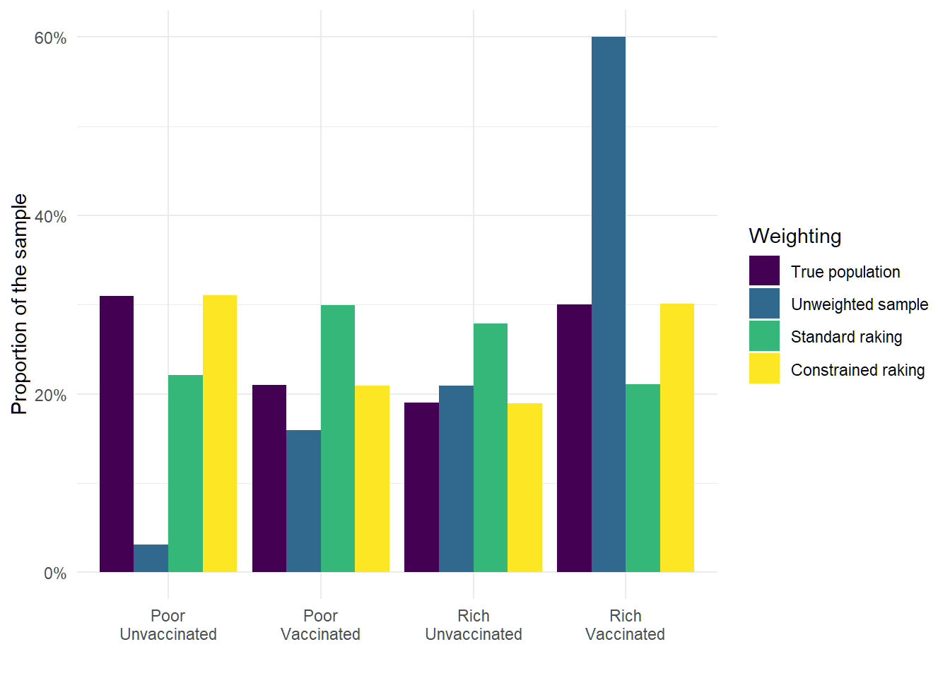
Figure 1: Proportion of people in each combination of wealth and vaccination status for the actual population, unweighted survey, using standard raking, and using raking with the minimum response rate fix.
This might seem almost unbelievable. We have somehow managed to exactly match the joint distribution of our variables without having access to any information about that joint distribution. The answer is that the constraint on the minimum weight is information about the joint distribution because it can rule out a large part of the possible space of joint distributions (because some joint distributions would contradict the known quantity of the response rate).
Now it is worth coming clean that I have shown the best case scenario here. If you know the column sums, row sums and one cell of a 2x2 matrix, you can fill in an exact solution for the rest of the cells. Because I set the response rate for rich vaccinated people to 100%, the minimum weight for that group is the correct weight for that cell.
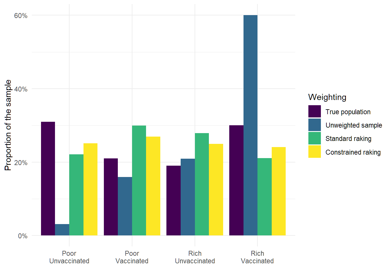
So let’s try a more realistic example. This time I’ve multiplied all of the subgroup response rates by 0.8 so that the rich vaccinated group’s response rate is 80% and the overall response rate is 40%.
| Vaccinated | Unvaccinated | |
|---|---|---|
| Rich | 80.0 | 44 |
| Poor | 30.4 | 4 |
The next plot shows that the minimum weight constraint no longer magically nails the cell proportions, but that we do see an improvement in the proportions when we include the constraint.
Is this useful in the real world?
So does this constraint gain us anything practically? Well, it represents a much stronger constraint when the response rate is higher, so this would have been a lot more valuable to discover 40 years ago. But this constraint is still likely to be useful in cases where we want to include lots of weighting factors. If you have 10 weighting targets, the standard raking algorithm is likely to heavily downweight some combinations of attributes. While it may be the case that these factors really do multiplicatively increase response rates, there is nothing in the standard raking algorithm that prevents it from proposing impossible joint distributions. Depending on the specifics of the data and population distributions, this constraint may provide a surprisingly large amount of information about the joint distribution.
There is one more advantage of this method: it increases weighting efficiency while reducing bias. Because the adjustment is theoretically motivated, it should reduce bias. But it also reduces the variance of the weights. This reduction is most obvious in the lower constraint, but the low weights are increased by proportionally taking away weight from all other observations. This means that the technique will also reduce extremely large weights.
Before anyone runs out to implement this, it will be necessary to extend the approach to account for stratification and selection probabilities (e.g. the fact that people in larger households have lower probabilities of selection, because the interviewer typically chooses a household member at random from a sampled address). My suspicion is that the constraint for \(i\)’s weight should be:
\[ \frac{FinalWeight_i}{SelectionWeight_i} > RR_{total} \]
but I haven’t actually proved this, so I could be way off (the goal of this blog is to post ideas that might turn out to be wrong after all).
This exercise also highlights the major limitation of non-probability data. Because non-probability data may have arbitrarily large levels of unobserved self-selection, there is no equivalent of a minimum weight in the non-probability case. For all we know, some non-probability survey respondents really may be hundreds of times more likely to participate than the average person.
So what do you think? Useful innovation, reinventing the wheel, or just an abstract mathematical finding without real applications?
Fortunately people in this fictional country never lie on surveys.↩︎